Figure 3.11 Petroleum supply/demand

Supply and demand. General approache

Fundamental to analyzing future economic conditions is supply and demand. Standard presentations of supply and demand fail to properly reflect the concepts of supply and demand. Most supply/demand forecasts plot supply/demand versus time, like those presented in Figure 3.11.

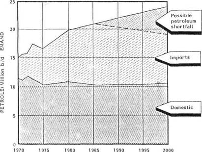
Figure 3.11 Petroleum supply/demand

Figure 3.11 distorts the supply/demand concept. A common phrase is "It depends on supply and demand." Supply and demand, in an economic context, are the result of many forces including price, costs, competition, and so on, not the cause.

Private companies produce minerals with the goal of making a profit. State owned companies also seek profits, but the profits are used for different purposes. A simple form for explaining supply is given in Equation 3.6.

Profit = (P)(Q)-(r)(K)-(w)(L) (3.6)

Where: Q = the quantity of mineral

P = the selling price

r = the price of capital

К = the amount of capital used

w = labor cost

L = the quantity of labor employed

Each product assumes capital and labor are combined in the optimum combination.

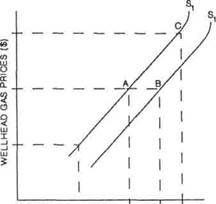
Supply describes the change in production (Q) as price (P) and costs (rK, wL) change. Supply curves are generated by holding costs constant, such as Figure 3.12. At $2.50 per MCF, about 10 TCF of gas is supplied. As gas price rises to $3.00 and $3.50 per MCF, 15 and 20 TCF of gas are supplied, respectively. After 20 TCF the supply curve, Si, which is the result of connecting these points become vertical, indicating that this is the capacity of production at a given point in time.

Curve S1 was generated by holding all forces affecting supply, such as costs, environmental issues, and so on, constant. Changing any of the values held constant shifts supply to the right or left, depending on whether costs increase or decrease. Curve S2 shows the impact of a cost decline on supply. At any given price level, producers are will­ing to supply more natural gas than they were when curve S1 was in effect. Reduced costs produce higher profits. At a price of $3.00, producers supply 18 TCF instead of 15 TCF. Supply curves like Fig­ure 3.11 are generated from Figure 3.12 by drawing a line between point AC or AB. If the points repre­sent different periods in time - say year t, t+1, and t+2 - connecting them produces a supply curve.

h 1'6 18 20

SUPPLY OF NATURAL GAS (TCF)

Figure 3.12 Natural gas supply curve

Demand, like supply, responds to several economic forces, including mineral price, income

level, price of substitutes, taste changes, and so on. Demand curves are most often generated by correlating historical demand levels with the price, in­come, expectations, etc. Expectations is a key con­cept in developing demand and supply curves, as ex­plained later. In a typical demand curve - demand varies inversely with price, or demand falls as prices rise. Figure 3.13 shows a relationship for gasoline and natural gas. Natural gas has a larger slope, in­dicating more substitutes exist for it. Gasoline is in­elastic, meaning that demand changes less than the corresponding change in price over the same period. Natural gas is elastic - a small price change leads to a larger demand change. The elasticity of natural gas occurs largely because of the number of sub­stitute fuels available for commercial use.