Finite element method

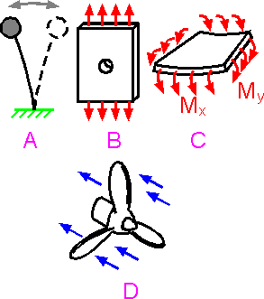The theories of elasticity, plasticity, plates and other analytical theories can be used to solve many engineering problems. Frequently, practical engineering problems cannot be solved analytically due to complexity of the structure's geometry and boundary conditions. The simple examples given in A, B and C can be solved to obtain inner stresses and displacements with analytical methods. More complicated geometries such as the propeller in example D is usually treated with a numerical method such as finite element method (FEM).

FEM is applied in the following manner:

1. Identify the problem, sketch the structure and loads.

2. Create the geometry with the FE package solid modeler or a CAD system.

3. Mesh the model.

4. Apply boundary conditions (constraints and loads) on the model.

5. Solve numerical equations.

6. Evaluate the results.

Steps 1, 2, 3, 4 are known as preprocessing, the solution of equations in step 5 is the processor and step 6 is considered postprocessing.
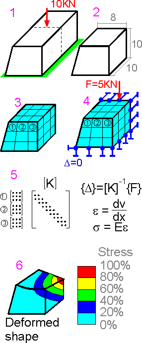
The FE model is normally subdivided into finite elements of a specific and simple shape. A typical 3D finite element may be a brick or a wedge with nodes representing the vertices. The displacement of the element is determined by nodal displacements and simple polynomial shape functions that describe the assigned shape of the element. The strains and stresses are calculated by the unknown nodal displacements. Once the nodal displacements are known, element stresses and strains can be calculated.

The most difficult and lengthy step of FEM is the preprocessing, or creating the finite element model. This step includes defining and generating the mesh and applying the correct loading and displacement boundary conditions. Automatic meshing is not always simple, especially in very small features or at the edges and corners. It can be difficult to apply boundary conditions that correspond to the real situation. However, FEM solvers that process the equations in step 5 work automatically and can be rather fast depending on the number of nodes. Powerful and robust visualization tools can allow for a very thorough analysis in step 6.

Degrees of freedoms

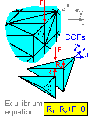Degrees of freedoms (DOF) are associated with each unknown nodal displacement. Each node of a 3D tetrahedral element has 3 DOF representing 3 translational motions. The equations of equilibrium are assembled in a matrix form. Problems with well over 100,000 DOF can be solved with a notebook computer.
Equilibrium equations refer to the equilibrium of each node in each direction:

The sum of all forces at an axis is equal to zero.

The sum of inner forces is equal to the sum of external forces.

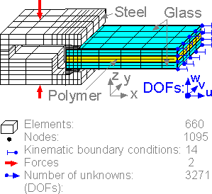The number of nodes is usually bigger than the number of elements for structured 3D models. The number of degrees of freedom is 3 times the number of nodes less the number of kinematic boundary conditions.

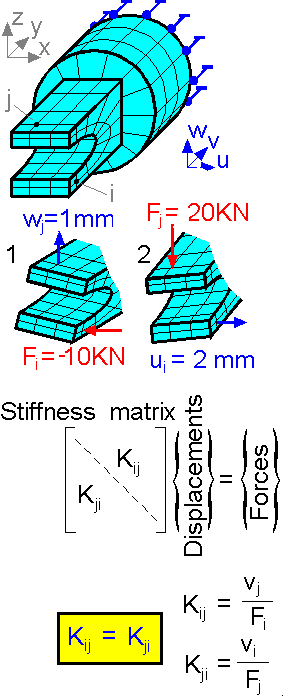The stiffness matrix [K] is the relationship between the vectors of nodal displacements {D} and forces {F}. The stiffness matrix is a diagonal-dominant matrix and is symmetric. It solves for nodal displacement given the loading scheme.