Capital budgeting and valuation with leverage

assume:Risk of the project to evaluate = risk of the firm; Debt/Equity remains constant.

WACC method: Compute unlevered Free Cash Flow, Compute WACC. Compute PV discounting FCF at WACC. This will be the value of levered firm (project). Additional assumptions: Market risk of the project is expected to be similar to that of the company’s other lines of business +

Debt/equity ratio is supposed to stay the same. By undertaking the new project the Company adds new assets with initial market value VL0 = $61.25 mln. Therefore, to maintain D/E constant the Company must add 0.5*61.25 = $30.625 mln in new debt. For this it can borrow $30.625 mln

Since only 28 mln is needed to fund the project, the rest 30.625 – 28 = 2.625 will be paid to shareholders as dividend (or share repurchase). We can ensure constant D/E further by properly adjusting debt each period. We call the amount of debt necessary for this “debt capacity”, denote Dt=d*VLt. Where d is D/(E+D). Here VLt – the project’s levered continuation value, i.e. VLt=(FCF_(t+1)+VL(t+1)) / (1+rwacc).Result: Firm (Enterprise) value. Use when leverage predetermined.

Adjusted Present Value (APV): Compute unlevered Free Cash Flow, Compute r_u– cost of capital for unlevered project (firm), Determine per period tax shield and it’s required return r_TS, Compute V_u and PV(Interest TS). Dr_D + Er_E = V^Ur_U + TSr_TS. But when D/E is kept constant, debt fluctuates with changes in VLt i.e. interest tax shield becomes risky and rTS = rU. =>!Use APV when the debt schedule is predetermined (e.g., constant level),!Use WACC when the debt ratio is constant. Result:Firm value (EV). Use when debt schedule is predetermined

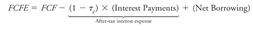
Flow-to-equity approach: Calculate Free Cash Flow to Equity, Difference from WACC and APV methods: here we compute the cash flow to equity of the levered firm; Compute their NPV using r_e as a discount rate. Result: Equity Value. Use when non-standard capital structure.

When estimating EV: in WACC use Net Debt rather than Debt, In APV use rU of the assets without excess cash, In APV use Net Debt to compute tax shield, In formulas for levering-unlevering betas or cost of equity (i.e., linking betaE with betaU or rE with rU) use Net Debt and rU of the assets without excess cash.

Taking into account the project-specific risk: Find firms in the market (comparables) whose whole business is similar to your project, and take their rU. If you don’t know r_E and r_D of the comparable firms, but know their β_E and β_D, then you use CAPM to find r_E and r_D, or you can directly compute βu=E/(E+D) β_E +D/(E+D) β_D (use the project’s D/(E+D)!!).

Assume you know rU and rd then if you need to achieve certain target D/(D+E) for your firm, then you need to solve simultaneously:(Dold+Dp)/(Dold+Dp+Eold+Ep) = D/(D+E)

Dp+Ep ≡ PVp = discounted FCF using WACC

WACC = (Ep/(Ep+Dp))*re + (Dp/(Ep+Dp))*(1-t)*rd

re is found from ru = (Ep/(Ep+Dp))*re + (Dp/(Ep+Dp))*rd

Unknowns Dp, Ep, WACC, re.

Relative valuation: If cash flow grows at constant rate g: V = CF1/(r-g) = cash flow multiple * CF1. Multiples: Earnings multiples: P/E, EV/EBITDA; Revenue multiples: P/S – price to sales ratio, EnterpV/S; Book Value multiples: P/BV – price to book value of equity, EV/BV; Sector-specific multiples: Value per user, Value per barrel of reserves…

People use growth-adjusted P/E ratio: PEG=(P/E)/g, where g is the expected growth in EPS. Then your P = (estimated PEG)*(your E)*(your g). Different capital structure: If a firm has higher leverage, then (ignoring effects of taxes and costs of fin distress): Earnings are lower (due to higher interest payments), Equity is lower too. In general, P/E: Decreases with leverage for low-growth or declining firms. Increases with leverage for high-growth firms. Thus, if your comparables have different leverage, it may be more meaningful to apply ratios that are based on the whole firm value, e.g., EV/Sales, EV/EBITDA; Volatility: Use forecasted earnings (if available), Use many comparables, Use EV/Sales - Sales never get too close to zero or negative.

Trading multiples: based on stock prices of publicly traded comparable firms; Transaction multiples: based on acquisition prices of comparable firms. Are transaction multiples normally higher or lower than trading multiples?

+ Control premium; + Synergies; + Operational improvements; – illiquidity discount; – “underdiversification” discount. => Overall, usually higher

Smart thoughts from HAs:

1. Equity is riskier with higher leverage (call option analog). The closer to exercise price, the greater the leverage. Debt and Equity become riskier as the firm gets closer to default.

2. Even though X’s debt is riskless (the firm will not default), the future growth of X’s debt is uncertain, so the exact amount of the future interest payments is risky. Assuming the future interest payments have beta equal to X’s unlevered beta, what is the present value of X’s tax shield? => The expected value of next year’s tax shield will be $250 × 40% = $100, and it will grow at a rate of 3%. But the exact amount of the tax shield is uncertain, since X may add new debt or repay some debt during the year, depending on their cash flows. This makes the actual amount of the tax shield risky (even though the debt itself is not). Since the beta of the tax shield due to debt is 1.11, the appropriate discount rate is 5% + 1.11 (11% – 5%) = 11.67%. conclude that PV(Interest Tax Shields) = 100/(0.1167-0.03)

3.