2018-02-14
 272
27221 That kind of intractability is sometimes called the "curse of dimensionality." Very large numbers of dimensions occur in practice. In mathematical finance, d can be the number of months in a 30-year mortgage.
Let us compare our d -dimensional integration problem with the Traveling Salesman Problem, a well-known example of a discrete combinatorial problem. The input is the location of n cities and the desired output is the minimal route that includes them all. The city locations are usually represented by a finite number of bits. Therefore, the input can be exactly entered into a digital computer. The complexity of this combinatorial problem is unknown, but is conjectured to be exponential in the number of cities, rendering the problem computationally intractable. In fact, many other combinatorial problems are conjectured to be intractable. This is a famous unsolved issue in computer science.
22 Many problems in scientific computation that involve multivariate functions turn out to be intractable in the worst-case setting; their complexity grows exponentially with the number of variables. Among the intractable problems are partial differential and integral equations, nonlinear optimization, nonlinear equations,9 and function approximation.
One can sometimes get around the curse of dimensionality by assuming that the function obeys a more stringent global condition than simply belonging to Fr. If, for example, one assumes that a function and its constraints are convex, then its nonlinear optimization requires only on the order of log(l/ε) evaluations of the function.
23 In general, information-based complexity assumes that the information concerning the mathematical model is partial, contaminated, and priced. In our integration example, the mathematical input is the integrand and the information is a finite set of function values. The information is partial because the integral cannot be recovered from the function values. For a partial differential equation, the mathematical input would be the functions specifying the boundary conditions. Usually, the mathematical input is replaced by a finite number of information operations—for example, functionals on the mathematical input or physical measurements that are fed into a mathematical model. Such information operations, in the real-number model, are permitted at cost с.
24 In addition to being partial, the information is often contaminated, for example, by measurement or rounding errors. If the information is partial or contaminated, one cannot solve the problem exactly. Finally, the information has a price. For example, the information needed for oil-exploration models is obtained by the explosive triggering of shock waves. With the exception of certain finite-dimensional problems, such as finding roots of systems of polynomial equations and doing matrix-algebra calculations, the problems typically encountered in scientific computation have information that is partial, contaminated, and priced.
25 Information-based complexity theory is developed over abstract spaces such as Banach and Hilbert spaces, and the applications typically involve multivariate functions. We often seek an optimal algorithm—one whose cost is equal or close to the complexity of the problem. Such endeavors have sometimes led to new methods of solution.
The information level
26 The reason why we can often obtain the complexity and an optimal algorithm for information-based complexity problems is that partial or contaminated information lets one make arguments at the information level. In combinatorial problems, by contrast, this information level does not exist, and we usually have to settle for conjectures and attempts to establish a hierarchy of complexities.
27 A powerful tool at the information level—one that's not available in discrete models of computation—is the notion of the radius of information, denoted by R. The radius of information measures the intrinsic uncertainty of solving a problem with a given body of information. The smaller this radius, the better the information. An ε-approximation can be computed if, and only if, R < ε.
The radius depends only on the problem being solved and the available information; it is independent of the algorithm. In every information-based complexity setting, one can define an R. (We've already touched on the worst-case setting above, and two additional settings are to come in the next section.) One can use R to define the "value of information," which I believe is preferable, for continuous problems, to Claude Shannon's entropy-based concept of "mutual information."
28 I present here a small selection of recent advances in the theory of information-based complexity: high-dimensional integration, path integrals, and the unsolvability of ill-posed problems.
29 Continuous multivariate problems are, in the worst-case setting, typically intractable with regard to dimension. That is to say, their complexity grow exponentially with increasing number of dimensions. One can try in two ways to attempt to break this curse of dimensionality: One can replace the ironclad worst-case ε-guarantee by a weaker stochastic assurance, or one can change the class of mathematical inputs. For high-dimensional integrals, both strategies come into play.
Monte Carlo
30 Recall that, in the worst-case setting, the complexity of d -dimensional integration is of order (l/ε)d/r. But the expected cost of the Monte Carlo method is of order (1/e)2, independent of d. This is equivalent to the common knowledge among physicists that the error of a Monte Carlo simulation decreases like
n-1/2. This expression for the cost holds even if r = 0. But there is no free lunch. Monte Carlo computation carries only a stochastic assurance of small error.
31 Another stochastic situation is the average-case setting. Unlike Monte Carlo randomization, this is a deterministic setting with an a priori probability measure on the space of mathematical inputs. The guarantee is only that the expected error with respect to this measure is at most ε and that the complexity is the least expected cost.
32 What is the complexity of integration in the average-case setting and where should the integrand be evaluated? This problem was open for some 20 years until it was solved by Wozniakowski in 1991. Even for the least smooth case r = 0, he proved that the average complexity is of order
ε-1 (log ε-1) (d-1)/2
and that the integrand should be evaluated at the points of a "low discrepancy sequence." Many such sequences are known in discrepancy theory, a much studied branch of number theory. Roughly speaking, a set of points has low discrepancy if a rather small number of points is distributed as uniformly as possible in the unit cube in d dimensions.
The integral of f is approximated by
n
1 Σ f (ti )
n i=1
In Monte Carlo computations, the points tt are chosen from a random distribution. If they constitute a low-discrepancy sequence, it is called a quasi—Monte Carlo computation. If we ignore the logarithmic factor in Wozniakowski's theorem, we see that a quasi-Monte Carlo computation costs only 1/ε, much less than the classic Monte Carlo method. If d is modest, one can indeed neglect the logarithmic factor. But in financial computations with d = 360, it looks ominous.
It was computer experiments by Spassimir Paskov on various financial computations that led to the surprising conclusion that quasi-Monte Carlo always beats ordinary Monte Carlo, often by orders of magnitude. Anargyros Papageorgiou and I have shown that with generalized Faure points, which form a particular kind of low-discreрanсу sequence, quasi-Monte Carlo computations can achieve accuracies of 1%—which is generally good enough for finance—with only 170 function evaluations.
33 A recent paper by Wozniakowski and Ian Sloan may explain this surprising power of quasi—Monte Carlo computation. They observe that many problems of mathematical finance are highly non-isotropic; that is to say, some dimensions are much more important than others. This is due, in part, to the discounted value of future money. They prove the existence of a quasi-Monte Carlo method whose worst-case cost is ε-p, independent of d, where p is no bigger than 2.
34 The quasi-Monte Carlo method also looks promising for problems in areas other than mathematical finance. For example, Papageorgiou and I have reported test results on a model integration problem suggested by integration problems in physics. Once again, quasi—Monte Carlo outperformed traditional Monte Carlo by a large factor, for d as large as 100.
35 Let me end this discussion with a caveat. There are many problems for which it has been established that randomization does not break intractability. One such instance, as shown by Greg Wasilkowski, is the problem of function approximation. How to characterize those problems for which randomization does breaks intractability remains an open question.
Path integrals
36 A new area of research of particular interest for physics is the complexity of path integrals. One can define a path integral
S(f) = ∫f(x) µ (dx),
x
where µ is a probability measure on an infinite-dimensional space X. Path integrals find numerous applications in quantum field theory, continuous financial mathematics, and the solution of partial differential equations. If to compute an ε-approximation to a path integral, the usual method is to approximate the infinite-dimensional integral by one of finite dimension, calculated by Monte Carlo.
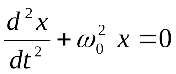
37 Here I briefly describe some very recent work on the complexity of path integral computation by Wasilkowski,Wozniakowski, and Leszek Plaskota. They considered a new algorithm for certain Feynman-Kac path integrals that concern the solution of the heat equation
d z(u, t) 1 d2 z(u,t)
dt = 2 du 2 + V(u) z(u,t), where z(u,0) = у(u)
with the Feynman-Kac integral
t
z(u, t) = ∫y (x(t) + u) exp (∫V (x (s) + u) ds) ω (d x),
с о
where V is a potential function, у is an initial condition function, С is the space of continuous functions, and ω is its Wiener measure. If V is sufficently smooth and у is constant, Alexandre Chorin's 1973 Monte Carlo algorithm yields a cost of ε-2,5 for stochastic assurance that the error is no more than ε.
38 By contrast, the new algorithm is deterministic. Its cost is only ε-2,5. And, for that bargain-basement price, one even gets a worst-case guarantee rather than just a stochastic assurance. But the new algorithm does have a drawback. It requires the calculation of certain coefficients given by weighted integrals. So one might say there's a precomputation cost that is not included in the advertised price of the algorithm.
39 Leaving that aside, ε-2,5 is an upper bound on the complexity of the problem. A lower bound has also been established and, for certain classes, the two bounds are essentially the same. So the complexity of the Feynman-Kac path integral problem is known and the new algorithm is essentially optimal. The results are, in fact, more general than I've indicated here. I just want to give the reader a taste of this work.
Ill-posed problems
40 As the final example, we look at ill-posed problems from the viewpoint of computability theory and information-based complexity, to show the power of analysis at work. In 1988, Marian Pour-El and Ian Richards established what Penrose has called "a rather startling result." Consider a wave equation for which the data provided at an initial time determines the solution at all later times. Then there exist computable initial conditions with the property that at a later time the field is not computable. A similar result holds for the backward heat equation. Both of these cases are examples of unbounded linear transformations, and they illustrate a theorem that tells us that an unbounded linear transformation can take computable inputs into non-computable outputs.
41 Pour-El and Richards devoted a large part of their monograph to proving this theorem by means of computability theory. An analogous result was established by Arthur Werschulz, by information-based complexity theory over the real numbers. Werschulz's proof, which is only about a page long, illustrates the power of analysis. As we shall see, his approach has several other advantages.
42 The classical theory of ill-posed problems was developed by Jacques Hadamard a century ago. Roughly speaking, a problem is ill-posed if small changes in the problem's specification can cause large changes in the solution. Hadamard felt there was something inherently wrong with trying to solve such problems. Given an ill-posed problem, one should attempt to reformulate it. There are, however, many important ill-posed problems that must be confronted in practice—for example, in remote sensing and computational vision.
43 Suppose we want to compute Lf, where L is a linear operator on the function f. The operator is said to be unbounded if, roughly speaking, the size of Lf is arbitrarily bigger than that of f, for some f. It is well known that Lf is ill-posed if, and only if, L is unbounded. The backward heat equation and the wave equation with an initial condition that is not twice differentiable are examples of problems whose solution is given by an unbounded linear operator. Werschulz assumed that the function f (which, for a differential equation, might be the initial condition) cannot be entered into a digital computer. So he discretized f by evaluating it at a finite number of points. Werschulz proved that, if the problem is ill-posed, it is impossible to compute an ε-approximation to the solution at finite cost for any ε, no matter how large. Thus the problem is unsolvable, which is a much stronger result than mere noncomputability.
44 But the best is yet to come. The notion of an unbounded linear operator is a worst-case concept. In information-based complexity, however, it is natural to consider average behavior. Werschulz places a measure on the inputs—for example, the initial conditions. He says a problem is well-posed, on average, if the expectation of Lf with respect to this measure is finite. Then it can be shown that every ill-posed problem is well-posed, on average, for every Gaussian measure and therefore solvable, on average. So we see that the unsolvability of ill-posed problems is a worst-case phenomenon. It melts away, on average, for reasonable measures.
45 I've tried here to provide a taste of some of the achievements of information-based complexity theory with the real-number model of computation. I invite the reader to look at some of the monographs cited in the references for other results and numerous open problems.
III .Vocabulary and Word Study
A. Vocabulary
1) импликация
1. implication n 2) включение
3) вовлечение
2. turing-type computer n машина Тьюринга
3. construct n конструкция
4. crux n затруднение, трудный вопрос
5. to deter v зд. откладывать
6. finite-state machine конечный автомат
7. lambda calculus лямбда счисление
8. running time 1) время прогона программы
2) продолжительность работы
3)машинное время, время обработки
9. to make available предоставлять
10.automata, pl
automaton sing автомат
11.unit cube единичный куб
12.to compete конкурировать
13.intractable с трудом поддающийся (зд.вычислению),
трудноразрешимый
14.mortgage ['mo:gidз] 1) ипотека
2) закладная
15.travelling salesman problem задача коммивояжёра
16.partial differential equation дифференциальное уравнение в частных
производных
17.curse n 1) проклятие
2) бич, бедствие
18.to contaminate v загрязнять
19.endeavor [in'devə] n 1) попытка, старание
2) стремление
20.discrepancy n 1) расхождение
2) рассогласование
3) отклонение
21.sequence n 1) последовательность, порядок следования
2) порядок чередования, очерёдность
22. discounted value of money текущая стоимость денег
23.caveat ['keiviæt] предостережение
24.computational model вычислительная модель
25.path integrals интегралы кривизны
Notes to the text
…phenomenon under consideration рассматриваемое явление
В Word study
1. Form nouns of the following verbs
N + ability → N
to compress to intract
to solve to compute
2. Form nouns of the following adjectives
Adj. + (c) ity → N
complex noncomputable
simple unsolvable
dimensional noncompatible
3. Improve your vocabulary
Make the following sentences complete by translating the words and phrases in brackets.
1) The physisist often chooses a continuous (вычислительная модель) for the phenomenon under consideration.
2) (Сложность вычисления) is a measure of the minimal (вычислительного ресурса) required to solve mathematically posed model.
3) (Реальная функция) of a real variable cannot be entered into (цифровую ВМ).
4) It requires (вычисления определённых коэффициентов) given by weighted integrals.
5) As the final (пример), we look at (неверно поставленные задачи) с точки зрения (теории вычисляемости) and information –based (сложности) to show (возможность анализа) в работе.